Excel tips

Useful advice for interacting with Excel for Spark

Optimize spreadsheets

Workbook construction

See Excel performance resources.
Minimize the number of worksheets.
Remove unnecessary external links or break them all together to reduce the chance of intended behaviors.
For large static tables, use paste values for any formulas to eliminate unnecessary calculations.
For calculations that are repeated, try to reference the calculation once rather than having it repeated many times in the workbook.
Try to keep the last cell on each Excel sheet as close to A1 as can to minimize file sizes.
Try to keep a cell consistently a string or a number. Where this tends to occur would be around:
- Formulas such as =IF(A2>B2, A2, "") should be replaced with =IF(A2>B2, A2, 0).
- Functions that trap errors such as IFERROR or IFNA.
- Data validation lists such as 1,2,3+.

Function usage

Avoid volatile functions as much as possible (INDIRECT, OFFSET, etc.).
Where possible, use sorted matches to improve performance for MATCH, VLOOKUP, XMATCH, XLOOKUP, etc.
- Ensure the data is sorted when using these parameters.
- Please be careful to exclude the header row from the lookup_array parameters.
For worksheets that use a large number of lookups or sums, consider using SUMIFS or XLOOKUP with an array of criteria or lookup_values. This provides Spark with the opportunity to optimize the calculations collectively for better performance, see the below sample file.
As an extension of the previous point, broader use of Dynamic array formulas is encouraged as it reduces repetitive formula entry in the workbook and is easier to optimize for performance.
Where Dynamic array formulas cannot be used, for columnar formula ranges, dragging the formulas down using the bottom right handle is better than copying and pasting. This is more easily identified as the same formula range in the Excel XML.
Whole-column references such as =VLOOKUP(B1, A:A, 1, FALSE) are not recommended.
Avoid using a multiplication instead of IF, e.g. =A1*B2*(C3=23) should be rewritten as =IF(C3=23,A1*B1) to minimize the number of mathematical operations.
Although Spark has extensive support for LAMBDA functions and helpers such as (BYCOL, BYROW, ISOMITTED, MAKEARRAY, MAP, REDUCE, SCAN), minimizing the use of these functions helps to improve performance.

11KB

Array optimized SUMIFS and XLOOKUP.xlsx

Open

Tips for optimizing performance obstructions (from Microsoft)

To improve general performance, we recommend reviewing Microsoft's Tips for optimizing performance obstructions. Key takeaways for Spark users include:

Avoid the use of forward reference to refer to cells that are to the right or below.
Minimize the use of circular references with iteration ("unroll" them instead).
Avoid links between workbooks.
Minimize links between worksheets.
Minimize the used range.
Be aware that whole-column references may not be as performant.
In lieu of multiple VLOOKUPs, consider using MATCH and multiple INDEX functions.
Keep array (a.k.a CSE/{}) formulas as small as possible, and consider using SUMPRODUCT instead.
Use comma syntax with SUMPRODUCT ; using it with * is less efficient, especially for arrays.
Avoid using Dfunctions like DSUM, DCOUNT, and DAVERAGE; use SUMIFS, COUNTIFS, and AVERAGEIFS instead.
Avoid using complicated formulas and functions in defined names.
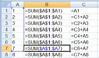
Avoid using the SUM function for long chains of cumulative sums, as shown in Column B, below. Over 1,000 rows, using the formulas in Column C requires about 498,000 fewer calculations!

Excel worksheet with three colums, column A has 8 cells with values 1 through 8, column B contains the formula `=SUM($A$1:$A1)` dragged down through all 8 cells. Cell C1 contains the formula `=A1` and C2 contains the formula `=C1+A2`

Define Named Ranges

Named Ranges enable cell(s) to be referred to as a Name in formulas. These are important for Spark because they are used to identify cells with certain behaviors like inputs and outputs.

Use the Name box

This creates a Name that can be used on every worksheet (Workbook scope).

Select the target cell(s).
Type the name in the Name Box.

Use the New Name dialog (Ctrl+Alt+F3)

The New Name dialog to edit the name scope and add a comment to the Name.

Select the target cell(s).
From the Ribbon, choose the Formulas tab and click Define Name.
The New Name dialog appears.

Use the Name Manager (Ctrl+F3)

The Name Manager can also be used to create, edit, delete, filter Names.

Select the target cell(s).
Click the Ribbon Formula tab and select Name Manager.
A list of the currently defined Names on the workbook can be edited.
Click New which presents the same dialog box as Excel tips.

Create from Selection (Ctrl+Shift+F3)

Create from Selection makes it very easy to define a large block of names using a formula.

Put the Xinput names beside the values.
Click the Ribbon Formula tab and select Create from Selection.
In this case because the proposed the names for the Named Ranges are on the left, choose Left column.
In this example, 4 Xinputs should be created.

Identify cells with Data Validation

From the Home tab in the ribbon, click the Find & Select menu and choose Data Validation. The cells with Data Validation will be selected. To make it easier to identify these cells, apply a color fill to the selected ranges.